Knowledge and anti-knowledge

Suppose knowledge has a non-infinitesimal value. Now imagine that you continuously gain evidence for some true proposition p, until your evidence is sufficient for knowledge. If you’re rational, your credence will rise continuously with the evidence. But if knowledge has a non-infinitesimal value, your epistemic utility with respect to p will have a discontinuous jump precisely when you attain knowledge. Further, I will assume that the transition to knowledge happens at a credence strictly bigger than 1/2 (that’s obvious) and strictly less than 1 (Descartes will dispute this).

But this leads to an interesting and slightly implausible consequence. Let T(r) be the epistemic utility of assigning evidence-based credence r to p when p is true, and let F(r) be the epistemic utility of assigning evidence-based credence r to p when p is false. Plausibly, T is a strictly increasing function (being more confident in a truth is good) and F is a strictly decreasing function (being more confident in a falsehood is bad). Furthermore, the pair T and F plausibly yields a proper scoring rule: whatever one’s credence, one doesn’t have an expectation that some other credence would be epistemically better.

It is not difficult to see that these constraints imply that if T has a discontinuity at some point 1/2 < r_K < 1, so does F. The discontinuity in F implies that as we become more and more confident in the falsehood p, suddenly we have a discontinuous downward jump in utility. That jump occurs precisely at r_K, namely when we gain what we might call “anti-knowledge”: when one’s evidence for a falsehood becomes so strong that it would constitute knowledge if the proposition were true.

Now, there potentially are some points where we might plausibly think that epistemic utility of having a credence in a falsehood takes a discontinuous downward jump. These points are:

• 1, where we become certain of the falsehood

• r_B, the threshold of belief, where the credence becomes so high that we count as believing the falsehood

• 1/2, where we start to become more confident in the falsehood p than the truth not-p

• 1 − r_B, where we stop believing not-p, and

• 0, where the falsehood p becomes an epistemic possibility.

But presumably r_K is strictly between r_B and 1, and hence r_K is no one of these points. Is it plausible to think that there is a discontinuous downward jump in epistemic utility when we achieve anti-knowledge by crossing the threshold r_K in a falsehood.

I am incline to say not. But that forces me to say that there is no discontinuous upward jump in epistemic utility once we gain knowledge.

On the other hand, one might think that the worst kind of ignorance is when you’re wrong but you think you have knowledge, and that’s kind of like the anti-knowledge point.

The dependence of evidence on prior confidence

Whether p is evidence for q will often depend on one’s background beliefs. This is a well-known phenomenon.

But here’s an interesting fact that I hadn’t noticed before: sometimes whether p is evidence for q depends on how confident one is in q.

The example is simple: let p be the proposition that all other reasonable people have confidence level around r in q. If r is significantly bigger than one’s current confidence level, then p tends to be evidence for q. If r is significantly smaller than one’s current confidence level, then p tends to be evidence against q.

Thresholds and precision

In a recent post, I noted that it is possible to cook up a Bayesian setup where you don’t meet some threshold, say for belief or knowledge, with respect to some proposition, but you do meet the same threshold with respect to the claim that after you examine a piece of evidence, then you will meet the threshold. This is counterintuitive: it seems to imply that you can know that you will have enough evidence to know something even though you don’t yet. In a comment, Ian noted that one way out of this is to say that beliefs do not correspond to sharp credences. It then occurred to me that one could use the setup to probe the question of how sharp our credences are and what the thresholds for things like belief and knowledge are, perhaps complementarily to the considerations in this paper.

For suppose we have a credence threshold r and that our intuitions agree that we can’t have a situation where:

1. we have transparency as to our credences,

2. we don’t meet r with respect to some proposition p, but

3. we meet r with respect to the proposition that we will meet the threshold with respect to p after we examine evidence E.

Let α > 0 be the “squishiness” of our credences. Let’s say that for one credence to be definitely bigger than another, their difference has to be at least α, and that to definitely meet (fail to meet) a threshold, we must be at least α above (below) it. We assume that our threshold r is definitely less than one: r + α ≤ 1.

We now want this constraint on r and α:

1. We cannot have a case where (a), (b) and (c) definitely hold.

What does this tell us about r and α? We can actually figure this out. Consider a test for p that have no false negatives, but has a false positive rate of β. Let E be a positive test result. Our best bet to generating a counterexample to (a)–(c) will be if the priors for p are as close to r as possible while yet definitely below, i.e., if the priors for p are r − α. For making the priors be that makes (c) easier to definitely satisfy while keeping (b) definitely satisfied. Since there are no false negatives, the posterior for p will be:

2. P(p|E) = P(p)/P(E) = (r−α)/(r−α+β(1−(r−α))).

Let z = r − α + β(1−(r−α)) = (1−β)(r−α) + β. This is the prior probability of a positive test result. We will definitely meet r on a positive test result just in case we have (r−α)/z = P(p|E) ≥ r + α, i.e., just in case

3. z ≤ (r−α)/(r+α).

(We definitely won’t meet r on a negative test result.) Thus to get (c) definitely true, we need (3) to hold as well as the probability of a positive test result to be at least r + α:

4. z ≥ r + α.

Note that by appropriate choice of β, we can make z be anything between r − α and 1, and the right-hand-side of (3) is at least r − α since r + α ≤ 1. Thus we can make (c) definitely hold as long as the right-hand-side of (3) is bigger than or equal to the right-hand-side of (4), i.e., if and only if:

5. (r+α)² ≤ r − α

or, equivalently:

6. α ≤ (1/2)((1+6r−3r²)^1/2−1−r).

It’s in fact not hard to see that (6) is necessary and sufficient for the existence of a case where (a)–(c) definitely hold.

We thus have our joint constraint on the squishiness of our credences: bad things happen if our credences are so precise as to make (6) true with respect to a threshold r for which we don’t want (a)–(c) to definitely hold. The easiest scenario for making (a)–(c) definitely hold will be a binary test with no false negatives.

We thus have our joint constraint on the squishiness of our credences: bad things happen if our credences have a level of precision equal to the right-hand-side of (6). What exactly that says about α depends on where the relevant threshold lies. If the threshold r is 1/2, the squishiness α is 0.15. That’s surely higher than the actual squishiness of our credences. So if we are concerned merely with the threshold being more-likely-than-not, then we can’t avoid the paradox, because there will be cases where our credence is definitely below the threshold and it’s definitely above the threshold that examination of the evidence will push us about the threshold.

But what’s a reasonable threshold for belief? Maybe something like 0.9 or 0.95. At r = 0.9, the squishiness needed for paradox is α = 0.046. I suspect our credences are more precise than that. If we agree that the squishiness of our credences is less than 4.6%, then we have an argument that the threshold for belief is more than 0.9. On the other hand, at r = 0.95, the squishiness needed for paradox is 2.4%. At this point, it becomes more plausible that our credences lack that kind of precision, but it’s not clear. At r = 0.98, the squishiness needed for paradox dips below 1%. Depending on how precise we think our credences are, we get an argument that the threshold for belief is something like 0.95 or 0.98.

Here's a graph of the squishiness-for-paradox α against the threshold r:

Note that the squishiness of our credences likely varies with where the credences lie on the line from 0 to 1, i.e., varies with respect to the relevant threshold. For we can tell the difference between 0.999 and 1.000, but we probably can’t tell the difference between 0.700 and 0.701. So the squishiness should probably be counted relative to the threshold. Or perhaps it should be correlated to log-odds. But I need to get to looking at grad admissions files now.

Knowing you will soon have enough evidence to know

Suppose I am just the slightest bit short of the evidence needed for belief that I have some condition C. I consider taking a test for C that has a zero false negative rate and a middling false positive rate—neither close to zero nor close to one. On reasonable numerical interpretations of the previous two sentences:

1. I have enough evidence to believe that the test would come out positive.

2. If the test comes out positive, it will be another piece of evidence for the hypothesis that I have C, and it will push me over the edge to belief that I have C.

To see that (1) is true, note that the test is certain to come out positive if I have C and has a significant probability of coming out positive even if I don’t have C. Hence, the probability of a positive test result will be significantly higher than the probability that I have C. But I am just the slightest bit short of the evidence needed for belief that I have C, so the evidence that the test would be positive (let’s suppose a deterministic setting, so we have no worries about the sense of the subjunctive conditional here) is sufficient for belief.

To see that (2) is true, note that given that the false negative rate is zero, and the false positive rate is not close to one, I will indeed have non-negligible evidence for C if the test is positive.

If I am rational, my beliefs will follow the evidence. So if I am rational, in a situation like the above, I will take myself to have a way of bringing it about that I believe, and do so rationally, that I have C. Moreover, this way of bringing it about that I believe that I have C will itself be perfectly rational if the test is free. For of course it’s rational to accept free information. So I will be in a position where I am rationally able to bring it about that I rationally believe C, while not yet believing it.

In fact, the same thing can be said about knowledge, assuming there is knowledge in lottery situations. For suppose that I am just the slightest bit short of the evidence needed for knowledge that I have C. Then I can set up the story such that:

3. I have enough evidence to know that the test would come out positive,

and:

4. If the test comes out positive, I will have enough evidence to know that I have C.

In other words, oddly enough, just prior to getting the test results I can reasonably say:

5. I don’t yet have enough evidence to know that I have C, but I know that in a moment I will.

This sounds like:

6. I don’t know that I have C but I know that I will know.

But (6) is absurd: if I know that I will know something, then I am in a position to know that the matter is so, since that I will know p entails that p is true (assuming that p doesn’t concern an open future). However, there is no similar absurdity in (5). I may know that I will have enough evidence to know C, but that’s not the same as knowing that I will know C or even be in a position to know C. For it is possible to have enough evidence to know something without being in a position to know it (namely, when the thing isn’t true or when one is Gettiered).

Still, there is something odd about (5). It’s a bit like the line:

7. After we have impartially reviewed the evidence, we will execute him.

Appendix: Suppose the threshold for belief or knowledge is r, where r < 1. Suppose that the false-positive rate for the test is 1/2 and the false-negative rate is zero. If E is a positive test result, then P(C|E) = P(C)P(E|C)/P(E) = P(C)/P(E) = 2P(C)/(1+P(C)). It follows by a bit of algebra that if my prior P(C) is more than r/(2−r), then P(C|E) is above the threshold r. Since r < 1, we have r/(2−r) < r, and so the story (either in the belief or knowledge form) works for the non-empty range of priors strictly between r/(2−r) and r.

Consequentialism and probability

Classic utilitarianism holds that the right thing to do is what actually maximizes utility. But:

1. If the best science says that drug A is better for the patient than drug B, then a doctor does the right thing by prescribing drug A, even if due to unknowable idiosyncracies of the patient, drug B is actually better for the patient.

2. Unless generalized Molinism is true, in indeterministic situations there is often no fact of the matter of what would really have happened had you acted otherwise than you did.

3. In typical cases what maximizes utility is saying what is true, but the right thing to do is to say what one actually thinks, even if that is not the truth.

These suggest that perhaps the right thing to do is the one that is more likely to maximize utility. But that’s mistaken, too. In the following case getting coffee from the machine is more likely to maximize utility.

4. You know that one of the three coffee machines in the breakroom has been wired to a bomb by a terrorist, but don’t know which one, and you get your morning coffee fix by using one of the three machines at random.

Clearly that is the wrong thing to do, even though there is a 2/3 probability that this coffee machine is just fine and utility is maximized (we suppose) by your drinking coffee.

This, in turn, suggests that the right thing to do is what has the highest expected utility.

But this, too, has a counterexample:

5. The inquisitor tortures heretics while confident that this maximizes their and others’ chance of getting into heaven.

Whatever we may wish to say about the inquisitor’s culpability, it is clear that he is not doing the right thing.

Perhaps, though, we can say that the inquisitor’s credences are irrational given his evidence, and the expected utilities in determining what is right and wrong need to be calculated according to the credences of the ideal agent who has the same evidence.

This also doesn’t work. First, it could be that a particular inquisitor’s evidence does yield the credences that they actually have—perhaps they have formed their relevant beliefs on the basis of the most reliable testimony they could find, and they were just really epistemically unlucky. Second, suppose that you know that all the coffee machines with serial numbers whose last digit is the same as the quadrilionth digit of π have been rigged to explode. You’ve looked at the coffee machine’s serial number’s last digit, but of course you have no idea what the quadrilionth digit of π is. In fact, the two digits are different. You did the wrong thing by using the coffee machine, even though the ideal agent’s expected utilities given your evidence would say that you did the right thing—for the ideal agent would know a priori what the quadrilionth digit of π is.

So it seems that there really isn’t a good thing for the consequentialist to say about this stuff.

The classic consequentialist might try to dig in their heels and distinguish the right from the praiseworthy, and the wrong from the blameworthy. Perhaps maximizing expected utility is praiseworthy, but is right if and only if it actually maximizes utility. This this still has problems with (2), and it still gets the inquisitor wrong, because it implies that the inquisitor is praiseworthy, which is also absurd.

The more I think about it, the more I think that if I were a consequentialist I might want to bite the bullet on the inquisitor cases and say that either the inquisitor is acting rightly or is praiseworthy. But as the non-consequentialist that I am, I think this is a horrible conclusion.

It can be rational to act as if one's beliefs were more likely true than the evidence makes them out to be

Consider this toy story about belief. It’s inconvenient to store probabilities in our minds. So instead of storing the probability of a proposition p, once we have evaluated the evidence to come up with a probability r for p, we store that we believe p if r ≥ 0.95, that we disbelieve p if r ≤ 0.05, and otherwise that we are undecided. (Of course, the “0.95” is only for the sake of an example.)

Now, here is a curious thing. Suppose I come across a belief p in my mind, having long forgotten the probability it came with, and I need to make some decision to which p is relevant. What probability should I treat p as having in my decision? A natural first guess is 0.95, which is my probabilistic threshold for belief. But that is a mistake. For the average probability of my beliefs, if I follow the above practice perfectly, is bigger than 0.95. For I don’t just believe things that have probability 0.95. I also believe things that have probability 0.96, 0.97 and even 0.999999. Intuitively, however, I would expect that there are fewer and fewer propositions with higher and higher probability. So, intuitively, I would expect the average probability of a believed proposition to be a somewhat above 0.95. How far above, I don’t know. And the average probability of a believed proposition is the probability that if I pick a believed proposition out of my mental hat, it will be true.

So even though my threshold for belief is 0.95 in this toy model, I should treat my beliefs as if they had a slightly higher probability than that.

This could provide an explanation for why people can sometimes treat their beliefs as having more evidence than they do, without positing any irrationality on their part (assuming that the process of not storing probabilities but only storing disbelieve/suspend/belief is not irrational).

Objection 1: I make mistakes. So I should take into account the fact that sometimes I evaluated the evidence wrong and believed things whose actual evidential probability was less than 0.95.

Response: We can both overestimate and underestimate probabilities. Without evidence that one kind of error is more common than the other, we can just ignore this.

Objection 2: We have more fine-grained data storage than disbelieve/suspend/believe. We confidently disbelieve some things, confidently believe others, are inclined or disinclined to believe some, etc.

Response: Sure. But the point remains. Let’s say that we add “confidently disbelieve” and “confidently believe”. It’ll still be true that we should treat the things in the “believe but not confidently” bin as having slightly higher probability than the threshold for “believe”, and the things in the “confidently believe” bin as having slightly higher probability than the threshold for “confidently believe”.

Divine simplicity and divine knowledge of contingent facts

One of the big puzzles about divine simplicity which I have been exploring is that of God’s knowledge of contingent facts. A sloppy way to put the question is:

1. How can God know p in one world and not know p in another, even though God is intrinsically the same in both worlds?

But that’s not really a question about divine simplicity, since the same is often true for us. Yesterday you knew that today the sun would rise. Yet there is a possible world w₂ which up to yesterday was exactly the same as our actual world w₁, but due to a miracle or weird quantum stuff, the sun did not rise today in w₂. Yesterday, you were intrinsically the same in w₁ and w₂, but only in w₁ did you know that today the sun would rise. For, of course, you can’t know something that isn’t true.

So perhaps the real question is:

2. How can God believe p in one world and not believe p in another, even though God is intrinsically the same in both worlds?

I wonder, however, if there isn’t a possibility of a really radical answer: it is false that God believes p in one world and not in another, because in fact God doesn’t have any beliefs in any world—he only knows.

In our case, belief seems to be an essential component of knowledge. But God’s knowledge is only analogical to our knowledge, and hence it should not be a big surprise if the constitutive structure of God’s knowledge is different from our knowledge.

And even in our case, it is not clear that belief is an essential component of knowledge. Anscombe famously thought that there was such a thing as intentional knowledge—knowledge of what you are intentionally doing—and it seems that on her story, the role played in ordinary knowledge by belief was played by an intention. If she is right about that, then an immediate lesson is that belief is not an essential component of knowledge. And in fact even the following claim would not be true:

3. If one knows p, then one believes or intends p.

For suppose that I intentionally know that I am writing a blog post. Then I presumably also know that I am writing a blog post on a sunny day. But I don’t intentionally know that I am writing a blog post on a sunny day, since the sunniness of the day is not a part of the intention. Instead, my knowledge is based in part on the intention to write a blog post and in part on the belief that it is a sunny day. Thus, knowledge of p can be based on belief that p, intention that p, or a complex combination of belief and intention. But once we have seen this, then we should be quite open to a lot of complexity in the structure of knowledge.

Of course, Anscombe might be wrong about there being such a thing as knowledge not constituted by belief. But her view is still intelligible. And its very intelligibility implies a great deal of flexibility in the concept of knowledge. The idea of knowledge without belief is not nonsense in the way that the idea of a fork without tines is.

The same point can be supported in other ways. We can imagine concluding that we have no beliefs, but we have other kinds of representational states, such as credences, and that we nonetheless have knowledge. We are not in the realm of tineless forks here.

Now, it is true that all the examples I can think of for other ways that knowledge could be constituted in us besides being based on belief still imply intrinsic differences given different contents (beyond the issues of semantic externalism due to twinearthability). But the point is just that knowledge is flexible enough concept, that we should be open to God having something analogous to our knowledge but without any contingent intrinsic state being needed. (One model of this possibility is here.)

When truth makes you do less well

One might think that being closer to the truth is guaranteed to get one to make better decisions. Not so. Say that a probability assignment p₂ is at least as true as a probability assignment p₁ at a world or situation ω provided that for every event E holding at ω we have p₂(E)≥p₁(E) and for every event E not holding at ω we have p₂(E)≤p₁(E). And say that p₂ is truer than p₁ provided that strict inequality holds in at least one case.

Suppose that a secret integer has been picked among 1, 2 and 3, and p₁ assigns the respective probabilities 0.5, 0.3, 0.2 to the three possibilities while p₂ assigns them 0.7, 0.1, 0.2. Then if the true situation is 1, it is easy to check that p₂ is truer than p₁. But now suppose that you are offered a choice between the following games:

• W₁: on 1 win $2, on 2 win $1100, and on 3 win $1000.

• W₂: on 1 win $1, on 2 win $1000, and on 3 win $1100

If you are going by p₁, you will choose W₁ and if you are going by p₂, you will choose W₂. But if the true number is 1, you would be better off picking W₁ (getting $2 instead of $1), so the truer probabilities will lead to a worse payoff. C’est la vie.

Say that a scoring rule for probabilities is truth-directed if it never assigns a poorer score for a truer set of probabilities. The above example shows that a proper scoring rule need not be truth-directed. For let s(p)(n) be the payoff you will get if the secret number is n and you make your decision between W₁ and W₂ rationally on the basis of probability assignment p (with ties broken in favor of W₁, say). Then s is a proper (accuracy) scoring rule but the above considerations show that s(p₂)(1)<s(p₁)(1), even though p₂ is truer at 1. In fact, we can get a strictly proper scoring rule that isn’t truth-directed if we want: just add a tiny multiple of a Brier accuracy score to s.

Intuitively we would want our scoring rules to be both proper and truth-directed. But given that sometimes we are pragmatically better off for having less true probabilities, it is not clear that scoring rules should be truth-directed. I find myself of divided mind in this regard.

How common is this phenomenon? Roughly it happens whenever the truer and less-true probabilities disagree on ratios of probabilities of non-actual events.

Proposition: Suppose two probability assignments are such that there are events E₁ and E₂ with probabilities strictly between 0 and 1, with ω₁ in neither event, and such that the ratio p₁(E₁)/p₁(E₂) is different from the ratio p₂(E₁)/p₂(E₂). Then there are wagers W₁ and W₂ such that p₁ prefers W₁ and p₂ prefers W₂, but W₁ pays better than W₂ at ω₁.

Truth directed scoring rules on an infinite space

A credence assignment c on a space Ω of situations is a function from the powerset of Ω to [0, 1], with c(E) representing one’s degree of belief in E ⊆ Ω.

An accuracy scoring rule s assigns to a credence assignment c on a space Ω and situation ω the epistemic utility s(c)(ω) of having credence assignment c when in truth we are in ω. Epistemic utilities are extended real numbers.

The scoring rule is strictly truth directed provided that if credence assignment c₂ is strictly truer than c₁ at ω, then s(c₂)(ω)>s(c₁)(ω). We say that c₂ is strictly truer than c₁ if and only if for every event E that happens at ω, c₂(E)≥c₁(E) and for every event E that does not happen at ω, c₂(E)≤c₁(E), and in at least one case there is strict inequality.

A credence assignment c is extreme provided that c(E) is 0 or 1 for every E.

Proposition. If the probability space Ω is infinite, then there is no strictly truth directed scoring rule defined for all credences, or even for all extreme credences.

In fact, there is not even a scoring rule that strictly truth directed when restricted to extreme credences, where an extreme credence is one that assigns 0 or 1 to every event.

This proposition uses the following result that my colleague Daniel Herden essentially gave me a proof of:

Lemma. If PX is the power set of X, then there is no function f : PX → X such that f(A)≠f(B) whenever A ⊂ B.

Now, we prove the Proposition. Fix ω ∈ Ω. Let s be a strictly truth directed scoring rule defined for all extreme credences. For any subset A of PΩ, define c_A to be the extreme credence function that is correct at ω at all and only the events in A, i.e., c_A(E)=1 if and only if ω ∈ E and E ∈ A or ω ∉ E and E ∉ A, and otherwise c_A(E)=0. Note that c_B is strictly truer than c_A if and only if A ⊂ B. For any subset A of PΩ, let f(A)=s(c_A)(ω).

Then f(A)<f(B) whenever A ⊂ B. Hence f is a strictly monotonic function from PPΩ to the reals. Now, if Ω is infinite, then the reals can be embedded in PΩ (by the axiom of countable choice, Ω contains a countably infinite subset, and hence PΩ has cardinality at least that of the continuum). Hence we have a function like the one the Lemma denies the existence of, a contradiction.

Note: This suggests that if we want strict truth directedness of a scoring rule, the scoring rule had better take values in a set whose cardinality is greater than that of the continuum, e.g., the hyperreals.

Proof of Lemma (essentially due to Daniel Herden): Suppose we have f as in the statement of the Lemma. Let ON be the class of ordinals. Define a function F : ON → A by transfinite induction:

• F(0)=f(⌀)

• F(α)=f({F(β):β < α}) whenever α is a successor or limit ordinal.

I claim that this function is one-to-one.

Let H_α = {F(δ):δ < α}.

Suppose F is one-to-one on β for all β < α. If α is a limit ordinal, then it follows that F is one-to-one on α. Suppose instead that α is a successor of β. I claim that F is one-to-one on α, too. The only possible failure of injectivity on α could be if F(β)=F(γ) for some γ < β. Now, F(β)=f(H_β) and F(γ)=f(H_γ). Note that H_γ ⊂ H_β since F is one-to-one on β. Hence f(H_β)≠f(H_γ) by the assumption of the Lemma. So, F is one-to-one on ON by transfinite induction.

But of course we can’t embed ON in a set (Burali-Forti).

Going against currently expected utilities

Today I am making an important decision between A and B. The expected utilities of A and B depend on a large collection of empirical propositions p₁, ..., p_n. Yesterday, I spent a long time investigating the truth values of these empirical propositions and I calculated the expected utility of A to be much higher than that of B. However, today I have forgotten the results of my investigations into p₁, ..., p_n, though I still remember that A had a higher expected utility given these investigations.

Having forgotten the results of my investigations into p₁, ..., p_n, my credences for them have gone back to some sort of default priors. Relative to these defaults, I know that B has higher expected utility than A.

Clearly, I should still choose A over B: I should go with the results of my careful investigations rather than the default priors. Yet it seems that I also know that relative to my current credences, the expected utility of B is higher than that of A.

This seems very strange: it seems I should go for the option with the smaller expected utility here.

Here is one possible move: deny that expected utilities are grounded in our credences. Thus, it could be that I still hold a higher expected utility for A even though a calculation based on my current credences would make B have the higher expected utility. I like this move, but it has a bit of a problem: I may well have forgotten what the expected utilities of A and B were, and only remember that A’s was higher than B’s.

Here is a second move: this is a case where I now have inconsistent credences. For if I keep my credences in p₁, ..., p_n at their default levels, I have a piece of evidence I have not updated my credences on, namely this: the expected utility of A is higher than that of B relative to the posterior credences obtained by gathering the now-forgotten evidence. What I should do is update my credences in p₁, ..., p_n on this piece of evidence, and calculate the expected utilities. If all goes well—but right now I don’t know if there is any mathematical guarantee that it will—then I will get a new set of credences relative to which A has a higher expected utility than B.

Credences and decision-theoretic behavior

Let p be the proposition that among the last six coin tosses worldwide that proceeded my typing the period at the end of this sentence, there were exactly two heads tosses. The probability of p is 6!/(2⁶⋅2!⋅4!) = 15/64.

Now that I know that, what is my credence in p? Is it 15/64? I don’t think so. I don’t think my credences are that precise. But if I were engaging in gambling behavior with amounts small enough that risk aversion wouldn’t come into play, now that I’ve done the calculation, I would carefully and precisely gamble according to 15/64. Thus, I do not think my decision-theoretic behavior reflects my credence—and not through any irrationality in my decision-theoretic behavior.

Here’s a case that makes the point perhaps even more strongly. Suppose I didn’t bother to calculate what fraction 6!/(2⁶⋅2!⋅4!) was, but given any decision concerning p, I calculate the expected utilities by using 6!/(2⁶⋅2!⋅4!) as the probability. Thus, if you offer to sell me a gamble where I get $19 if p is true, I would value the gamble at $19⋅6!/(2⁶⋅2!⋅4!)$, and I would calculate that quantity as $4.45 without actually calculating 6!/(2⁶⋅2!⋅4!). (E.g., I might multiply 19 by 6! first, then divide by 2⁶⋅2!⋅4!.) I could do this kind of thing fairly mechanically, without noticing that $4.45 is about a quarter of $19, and hence without having much of an idea as to where 6!/(2⁶⋅2!⋅4!) lies in the 0 to 1 probability range. If I did that, then my decision-theoretic behavior would be quite rational, and would indicate a credence of 15/64 in p, but in fact it would be pretty clearly incorrect to say that my credence in p is 15/64. In fact, it might not even be correct to say that I assigned a credence less than a half to p.

I could even imagine a case like this. I make an initial mental estimate of what 6!/(2⁶⋅2!⋅4!) is, and I mistakenly think it’s about three quarters. As a result, I am moderately confident in p. But whenever a gambling situation is offered to me, instead of relying on my moderate confidence, I do an explicit numerical calculation, and then go with the decision recommended to me by expected utility maximization. However, I don’t bother to figure out how the results of these calculations match up with what I think about p. If you were to ask me, I would say that p is likely true. But if you were to offer me a gamble, I would do calculations that better fit with the hypothesis of my having a credence close to a quarter. In this case, I think my real credence is about three quarters, but my rational decision-theoretic behavior is something else altogether.

Furthermore, there seems to me to be a continuum between my decision-theoretic behavior coming from mental calculation, pencil-and-paper calculation, the use of a calculator or the use of a natural language query system that can be asked “What is the expected utility of gambling on exactly two of six coin tosses being heads when the prize for being right is $19?” (a souped up Wolfram Alpha, say). Clearly, the last two need not reflect one’s credences. And by the same token, I think that neither need the first two.

All this suggests to me that decision-theoretic behavior lacks the kinds of tight conceptual connection to credences that people enamored of representation theorems like.

Valuations and credences

One picture of credences is that they are derived from agents’ valuations of wagers (i.e., previsions) as follows: the agent’s credence in a proposition p is equal to the agent’s valuation of a gamble that pays one unit if p is true and 0 units if p false.

While this may give the right answer for a rational agent, it does not work for an irrational agent. Here are two closely related problems. First, note that the above definition of credences is dependent on the unit system in which the gambles are denominated. A rational agent who values a gamble that pays one dollars on heads and zero dollars otherwise at half a dollar will also value a gamble that pays one yen on heads and zero yen otherwise at half a yen, and we can attribute a credence of 1/2 in heads to the agent. In general, the rational agent’s valuations will be invariant under affine transformations and so we do not have a problem. But Bob, an irrational agent, might value the first gamble at $0.60 and the second at 0.30 yen. What, then, is that agent’s credence in heads?

If there were a privileged unit system for utilities, we could use that, and equate an agent’s credence in p with their valuation of a wager that pays one privileged unit on p and zero on not-p. But there are many units of utility, none of them privileged: dollars, yen, hours of rock climbing, glazed donuts, etc.

And even if there were a privileged unit system, there is a second problem. Suppose Alice is an irrational agent. Suppose Alice has two different probability functions, P and Q. When Alice needs to calculate the value of a gamble that pays exactly one unit on some proposition and exactly zero units on the negation of that proposition, she uses classical mathematical expectation based on P. When Alice needs to calculate the value of any other gamble—i.e., a gamble that has fewer than or more than two possible payoffs or a gamble that has two payoffs but at values other than exactly one or zero—she uses classical mathematical expectation based on Q.

Then the proposed procedure attributes to Alice the credence function P. But it is in fact Q that is predictive of Alice’s behavior. For we are never in practice offered gambles that have exactly two payoffs. Coin-toss games are rare in real life, and even they have more than two payoffs. For instance, suppose I tell you that I will give you a dollar on heads and zero otherwise. Well, a dollar is worth a different amount depending on when exactly I give it to you: a dollar given earlier is typically more valuable, since you can invest it for longer. And it’s random when exactly I will pay you. So on heads, there are actually infinitely many possible payoffs, some slightly larger than others. Moreover, there is a slight chance of the coin landing on the edge. While that eventuality is extremely unlikely, it has a payoff that’s likely to be more than a dollar: if you ever see a coin landing on edge, you will get pleasure out of telling your friends about it afterwards. Moreover, even if we were offered a gamble that had exactly two payoffs, it is extremely unlikely that these payoffs would be exactly one and zero in the privileged unit system.

The above cases do not undercut a more sophisticated story about the relationship between credences and valuations, a story on which one counts as having the credence that would best fit one’s practical valuations of gambles with two-values, and where there is a tie, one’s credences are underdetermined or interval-valued. In Alice’s case, for instance, it is easy to say that Q best fits the credences, while in Bob’s case, the credence for heads might be a range from 0.3 to 0.6.

But we can imagine a variant of Alice where she uses P whenever she has a gamble that has only two payoffs, and she uses Q at all other times. Since in practice two-payoff gambles don’t occur, she always uses Q. But if we use two-payoff gambles to define credences, then Alice will get P attributed to her as her credences, despite her never using P.

Can we have a more sophisticated story that allows credences to be defined in terms of valuations of gambles with more payoffs than two? I doubt it. For there are multiple ways of relating a prevision to a credence when we are dealing with an inconsistent agent, and none of them seem privileged. Even my favorite way, the Level Set Integral, comes in two versions: the Split and Shifted versions.

Strict propriety of credential scoring rules

An (inaccuracy) scoring rule measures how far a probabilistic forecast lies from the truth. Thus, it assigns to each forecast p a score s(p) which is a [0, ∞]-valued random variable varying over the probability space Ω that measures distance from truth. Let’s work with finite probability spaces and assume all the forecasts are consistent probability functions.

A rule s is proper provided that E_ps(p)≤E_ps(q) for any probability functions p and q, where E_pf = ∑_ω∈Ωp({ω})f(ω) is the expectation of f according to p, using the convention that 0 ⋅ ∞ = 0. Propriety is the very reasonable condition that whatever your forecast, according to your forecast you don’t expect any other other specific forecast to be better—if you did, you’d surely switch to it.

A rule is strictly proper provided that E_ps(p)<E_ps(q) whenever p and q are distinct. It says that by the lights of your forecast, your forecast is better than any other. It is rather harder to intuitively justify strict propriety.

A very plausible condition is continuity: your score in every possible situation ω ∈ Ω depends continuously on your probability assignment.

Last week while having a lot of time on my hands while our minivan was having an oil change, I got interested in the question of what kinds of failures of strict propriety can be exhibited by a continuous proper scoring rule. It is, of course, easy to see that one can have continuous proper scoring rules that aren’t strictly proper: for instance, one can assign the same score to every forecast. Thinking about this and other examples, I conjectured that the only way strict propriety can fail in a continuous proper scoring rule (restricted to probability functions) is by assigning the same score to multiple forecasts.

Last night I found what looks to be a very simple proof of the conjecture: Assuming the proof is right (it still looks right this morning), if s is a continuous proper scoring rule defined on the probabilities, and E_ps(p)=E_ps(q), then s(p)=s(q) (everywhere in Ω).

Given this, the following follows:

• A continuous scoring rule defined on the probabilities is strictly proper if and only if it is proper and fine-grained,

where a scoring rule is fine-grained provided that it is one-to-one on the probabilities: it assigns different scores to different probabilities. (I mean: if p and q are different, then there is an ω ∈ Ω such that s(p)(ω)≠s(q)(ω).)

But fine-grainness seems moderately plausible to me: a scoring rule is insufficiently “sensitive” if it assigns the same score to different consistent forecasts. So we have an argument for strict propriety, at least as restricted to consistent probability functions.

Expected utility and inconsistent credences

Suppose that we have a utility function U and an inconsistent credence function P, and for simplicity let’s suppose that our utility function takes on only finitely many values. The standard way of calculating the expected utility of U with respect to P is to look at all the values U can take, multiply each by the credence that it takes that value, and add:

1. E(U)=∑_yyP(U = y).

Call this the Block Way or Lebesgue Sums.

Famously, doing this leads to Dutch Books if the credence function fails additivity. But there is another way to calculate the expected utility:

2. E(U)=∫₀^∞P(U > y)dy − ∫_−∞⁰P(U < y)dy.

Call this the Level Set Way, because sets of points in a space where some function like U is bigger or smaller than some value are known as level sets.

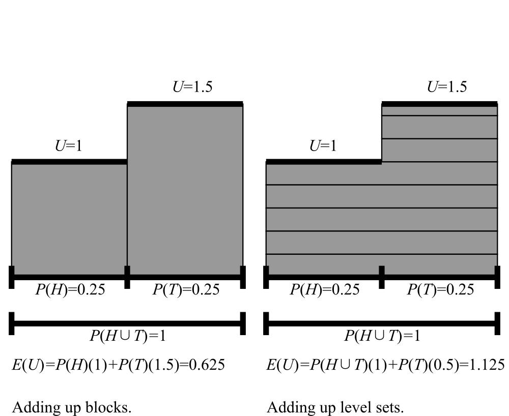
Here is a picture of the two ways:

On the Block Way, we broke up the sample space into chunks where the utility function is constant and calculated the contribution of each chunk using the inconsistent credence function, and then added. On the Level Set Way, we broke it up into narrow strips, and calculated the contribution of each strip, and then added.

It turns out that if the credence function P is at least monotone, so that P(A)≤P(B) if A ⊆ B, a condition strictly weaker than additivity, then an agent who maximizes utilities calculated the Level Set Way will not be Dutch Booked.

Here is another fact about the Level Set Way. Suppose two credence functions U₁ and U₂ are certain to be close to each other: |U₁ − U₂|≤ϵ everywhere. Then on the Block Way, their expected utilities may be quite far apart, even assuming monotonicity. On the other hand, on the Level Set Way, their expected utilities are guaranteed to be within ϵ, too. The difference between the two Ways can be quite radical. Suppose a coin is tossed, and the monotone inconsistent credences are:

• heads: 0.01

• tails: 0.01

• heads-or-tails: 1

• neither: 0

Suppose that U₁ says that you are paid a constant $100 no matter what happens. Both the Block Way and the Level Set Way agree that the expected utility is $100.
But now suppose that U₂ says you get paid $99 on heads and $101 on tails. Then the Block Way yields:

• E(U₂)=0.01 ⋅ 99 + 0.01 ⋅ 101 = 1

while the Level Set Way yields:

• E(U₂)=1 ⋅ 99 + 0.01 ⋅ 2 = 99.02

Thus, the Block Way makes the expected value of U₂ ridiculously small, and far from that of U₁, while the Level Set Way is still wrong—after all, the credences are stupid—but is much closer.

So, it makes sense to think of the Level Set Way as harm reduction for those agents whose credences are inconsistent but still monotone.

That said, many irrational agents will fail monotonicity.

Do inconsistent credences lead to Dutch Books?

It is said that if an agent has inconsistent credences, she is Dutch Bookable. Whether this is true depends on how the agent calculates expected utilities. After all, expected utilities normally are Lebesgue integrals over a probability measure, but the inconsistent agent’s credences are not a probability measure, so strictly speaking there is no such thing as a Lebesgue integral over them.

Let’s think how a Lebesgue integral is defined. If P is a probability measure and U is a measurable function on the sample space, then the expected value of U is defined as:

1. E(U)=∫₀^∞P(U > y)dy − ∫_−∞⁰P(U < y)dy

where the latter two integrals are improper Riemann integrals and where P(U > y) is shorthand for P({ω : U(ω)>y}) and similarly for P(U < y).

Now suppose that P is not a probability measure, but an arbitrary function from the set of events to the real numbers. We can still define the expected value of U by means of (1) as long as the two Riemann integrals are defined and aren’t both ∞ or both −∞.

Now, here is an easy fact:

Proposition: Suppose that P is a function from a finite algebra of events to the non-negative real numbers such that P(∅)=0. Suppose that U is a measurable (with respect to the finite algebra) function such that (a) P(U > y)=0 for all y > 0 and (b) P(U < 0)>0. Then if E(U) is defined by (1), we have E(U)<0.

Proof: Since the algebra is finite and U is measurable, U takes on only finitely many values. If y₀ is the largest of its negative values, then P(U < 0)=P(U < y) for any negative y > y₀, and hence ∫_−∞⁰P(U < y)dy ≥ |y₀|P(U < 0)>0 by (b), while ∫₀^∞P(U > y)dy by (a). □

But then:

Corollary: If P is a function from a finite algebra of events on the samples space Ω to the non-negative real numbers with P(∅)=0 and P(Ω)>0, then an agent who maximizes expected utility with respect to the credence assignment P as computed via (1) and starts with a baseline betting portfolio for which the utility is zero no matter what happens will never be Dutch Boooked by a finite sequence of changes to her portfolio.

Proof: The agent starts off with a portfolio with a utility assignment U₀ where P(U₀ > y)=0 for all y > 0 and P(U₀ < y)=0 for all y < 0, and hence once where E(U₀)=0 by (1). If the agent is in a position where the expected utility based on her current portfolio is non-negative, she will never accept a change to the portfolio that turns the portfolio’s expected utility negative, as that would violated expected utility maximization. By mathematical induction, no finite sequence of changes to her portfolio will turn her expected utility negative. But if a portfolio is a Dutch Book then the associated utility function U is such that P(U < 0)=P(Ω)>0 and P(U > y)=0 for all y > 0. Hence by the Proposition, E(U)<0, and hence a Dutch Book will not be accepted at any finite stage. □

Note that the Corollary does assume a very weak consistency in the credence assignment: negative credences are forbidden, impossible events get zero credence, and necessary events get non-zero credence.

Additionally, the Corollary does allow for the possibility of what one might call a relative Dutch Book, i.e., a change between portfolios that loses the agent money no matter what. The final portfolio won’t be a Dutch Book relative to the initial baseline portfolio, of course.

Note, however, that we don’t need consistency to get rid of relative Dutch Books. Adding the regularity assumption that P(A)>0 for all non-empty A and the monotonicity condition that if A ⊂ B then P(A)<P(B) is all we need to ensure the agent will never accept even a relative Dutch Book. For regularity plus monotonicity ensures that a relative Dutch Book always decreases expected utility as defined by (1). But these conditions are not enough to rule out all inconsistency. For instance, if in the case of the flip of a single coin I assign probability 1 to heads-or-tails, probability 0.8 to heads, probability 0.8 to tails, and probability 0 to the empty event, then my assignment is patently inconsistent, but satisfies all of the above assumptions and hence is neither absolutely nor relatively Dutch Bookable.

How does all this cohere with the famous theorems about inconsistent credence assignments being Dutch Bookable? Simple: Those theorems define expected utility for inconsistent credences differently. Specifically, they define expected utility as ∑_iU_iP(E_i) where the E_i partition the sample space such that on E_i the utility has the constant value U_i. But that’s not the obvious and direct generalization of the Lebesgue integral!

I vaguely recall hearing something that suggests to me that this might be in the literature.

Also, I slept rather poorly, so I could be just plain mistaken in the formal stuff.

A measure of sincerity

On a supervaluationist view of vagueness, a sentence such as “Bob is bald” corresponds to a large number of perfectly precise propositions, and is true (false) if and only if all of these propositions are true (false). This is plausible as far as it goes. But it seems to me to be very natural to add to this a story about degrees of truth. If Bob has one hair, and it’s 1 cm long, then “Bob is bald” is nearly true, even though some precisifications of “Bob is bald” (e.g., that Bob has no hairs at all, or that his total hair length is less than 0.1 cm) are false. Intuitively, the more precisifications are true, the truer the vague statement:

1. The degree of truth of a vague statement is the proportion of precisifications that are true.

But for technical reasons, (1) doesn’t work. First, there are infinitely many precisifications of “Bob is bald”, and most of the time the proportion of precisifications that are true will be ∞/∞. Moreover, not all precisifications are equally good. Let’s suppose we somehow reduce the precisifications to a finite number. Still, let’s ask this question: If Bob is an alligator is Bob bald? This seems vague, even though the precisifications of “Bob is bald” that require Bob to be the sort of thing that has hair seem rather better. But for any precisification that requires Bob to be a hairsute kind of thing, there is one that does not. And so if Bob is an alligator, he is bald according to exactly half of the precisifications, and hence by (1) it would be half-true that he is bald. And that seems too much: if Bob is an alligator, he is closer to being non-bald than bald.

A better approach seems to me to be this. A language assigns to each sentence s a set of precisifications and a measure m_s on this set with total measure 1 (i.e., technically a probability measure, but it does not represent chances or credences). The degree of truth of a sentence, then, is the measure of the subset of precisifications that are actually true.

Suppose now that we add to our story a probability measure P representing credences. Then we can form the interesting quantity E_P(m_s) where E_P is the expected value with respect to P. If s is non-vague, then E_P(m_s) is just our credence for s. Then E_P(m_s) is an interesting kind of “sincerity measure” (though it may not be a measure in the mathematical sense) that combines both how true a statement is and how sure we are of it. When E_P(m_s) is close to 1, then it is likely that s is nearly true, and when it is close to 0, then it is likely that s is nearly false. But when it is close to 1/2, there are lots of possibilities. Perhaps, s is nearly certain to be half-true, or maybe s is either nearly true or nearly false with probabilities close to 1/2, and so on.

This is not unlikely worked out, or refuted, in the literature. But it was fun to think about while procrastinating grading. Now time to grade.

Credence and belief

For years, I’ve been inclining towards the view that belief is just high credence, but this morning the following argument is swaying me away from this:

1. False belief is an evil.

2. High credence in a falsehood is not an evil.

3. So, high credence is not belief.

I don’t have a great argument for (1), but it sounds true to me. As for (2), my argument is this: There is no evil in having the right priors, but having the right priors implies lots high credences in falsehoods.

Maybe I should abandon (1) instead?

Erring on the side of moderation leads to erring on the side of extremism, at least epistemically

One might think that having a less extreme (i.e., further from 0 and 1, and closer to 1/2) credence than is justified by the evidence is pretty safe epistemically. So, if one wants to be safe, one should move one’s credences closer to 1/2: moderation is safer than extremism.

But if one is to be consistent, this doesn’t work. For instance, suppose that the evidence points to clearly independent hypotheses A and B each having probability 0.6, but in the name of safety one assigns them 0.5. Then consistency requires one to assign their conjunction 0.5 × 0.5 = 0.25, whereas the evidence pointed to their conjunction having probability 0.6 × 0.6 = 0.36. In other words, by being more moderate about A and B, one is more extreme about their conjunction.

In other words, once we have done our best in evaluating all the avilable evidence, we should go with the credence the evidence points to, rather than adding fudge factors to make our credences more moderate. (Of course, in particular cases, the existence of some kind of a fudge factor may be a part of the available evidence.)

Assertion threshold

Some people like me assert things starting with a credence like 0.95. Other people are more restrictive and only assert at a higher credence, say 0.98. Is there a general fact as to what credence one should assert at? I am not sure. It seems to me that this is an area where decent and reasonable people can differ, within some range (no one should assert at 0.55, and no one should refuse to assert at 0.999999999). Maybe what is going on here is that there is an idiolect-like phenomenon at the level of illocutionary force. And somehow we get by with these different idiolects, but with some inductive heuristics like “Alice only speaks when she is quite sure”.

More on credences of randomly chosen propositions

For a number of years I’ve been interested in what one might call “the credence of a random proposition”. Today, I saw that once precisely formulated, this is pretty easy to work out in a special case, and it has some interesting consequences.

The basic idea is this: Fix a particular rational agent and a subject matter the agent thinks about, and then ask what can be said about the credence of a uniformly randomly chosen proposition on that subject matter. The mean value of the credence will be, of course, 1/2, since for every proposition p, its negation is just as likely to be chosen.

It has turned out that on the simplifying assumption that all the situations (or worlds) talked about have equal priors, the distribution of the posterior credence among the randomly chosen propositions is binomial, and hence approximately normal. This was very easy to show once I saw how to formulated the question. But it still wasn’t very intuitive to me as to why the distribution of the credences is approximately normal.

Now, however, I see it. Let μ be any probability measure on a finite set Ω—say, the posterior credence function on the set of all situations. Let p be a uniformly chosen random proposition, where one identifies propositions with subsets of Ω. We want to know the distribution of μ(p).

Let the distinct members (“situations”) of Ω be ω₁, ..., ω_n. A proposition q can be identified with a sequence q₁, ..., q_n of zeroes and/or ones, where q_i is 1 if and only if ω_i ∈ q (“q is true in situation ω_i”). If p is a uniformly chosen random proposition, then p₁, ..., p_n will be independent identically distributed random variables with P(p_i = 0)=P(p_i = 1)=1/2, and p will be the set of the ω_i for which p_i is 1.

Then we have this nice formula:

1. μ(p)=μ(ω₁)p₁ + ... + μ(ω_n)p_n.

This formula shows that μ(p) is the sum of independent random variables, with the ith variable taking on the possible values 0 and μ(ω_i) with equal probability.

The special case in my first post today was one where the priors for all the ω_i are equal, and hence the non-zero posteriors are all equal. Thus, as long as there are lots of non-zero posteriors—i.e., as long as there is a lot we don’t know—the posterior credence is by (1) a rescaling of a sum of lots of independent identically distributed Bernoulli random variables. That is, of course, a binomial distribution and approximately a normal distribution.

But what if we drop the assumption that all the situations have equal priors? Let’s suppose, for simplicity, that our empirical data precisely rules out situations ω_m + 1, ..., ω_n (otherwise, renumber the situations). Let ν be the prior probabilities on Ω. Then μ is directly proportional to ν on {ω₁, ..., ω_m} and is zero outside of it, and:

2. μ(p)=c(ν(ω₁)p₁ + ... + ν(ω_m)p_m)

where c = 1/(ν(ω₁)+.... + ν(ω_m)). Thus, μ(p) is the sum of m independent but perhaps no longer identically distributed random variables. Nonetheless, the mean of μ(p) will still be 1/2 as is easy to verify. Moreover, if the ν(ω_i) do not differ too radically among each other (say, are the same order of magnitude), and m is large, we will still be close to a normal distribution by the Berry-Esseen inequality and its refinements.

In other words, as long as our priors are not too far from uniform, and there is a lot we don’t know (i.e., m is large), the distribution of credences among randomly chosen propositions is approximately normal. And to get estimates on the distribution of credences, we can make use of the vast mathematical literature on sums of independent random variables. This literature is available even without the "approximate uniformity" condition on the priors (which I haven't bothered to formulate precisely).